Satellite Process

Satellite Image Processing

The goal of this step is to prepare the satellite images for correlation analysis with a larger road map. We approach this problem by attempting to processing the images such that they look as similar as possible to the output of our road map processing. This page first describes each of the processing steps used in our final implementations followed by descriptions of other processes with which we experimented or more advanced methods that we believe may avoid some of the limitations of our approach

Imagery Dataset

For developing our digital signal processing techniques, we use the orthoimagery dataset provided by the United States Geological Survery. This data provides the following advantages [1]:

Multispectral: some images come with near-infrared layers in addition to the traditional red, green, and blue layers.
High Resolution: our images have a resolution of 1-4 ft/pixel
Corrections: supplier has made corrections for terrain relief, sensor geometry, and camera tilt. This allows for the images to be overlaid on road maps without distortion
Metadata: all images come with data including GPS coordinates, resolution, and more

To limit the variability in input images, we have also reduced our inputs to come from a single dataset (200809_san_francisco_ca_0x3000m_utm_clr). This allows us to tune our filters to the properties of these images and assume a certain degree of consistency in inputs. An sample images of San Francisco are shown in Figure 1.

1/8

Figure 1: Sample Aerial Image of San Francisco

Color Space Transformation

The downloaded images are stored with pixel colors in the RGB color-space, meaning each color is represented by a 3D space where the dimensions represent intensity of red, green, and blue respectively. We found subsequent filtering to be more easily defined if the colors were represented in an HSV color-space. This color-space is again three dimensional with each direction representing hue, saturation, and value (brightness) respectively. A visualization of these is shown in Figure 2.

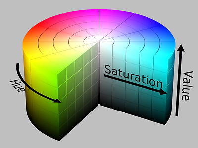
Figure 2.1: RGB Color Space [2]

Figure 2.2: HSV Color Space [3]

Color Threshold Filter

Once the colors were represented conveniently, we applied a color filter. This filter makes the assumption that roads lie within a certain range of grays and is tuned to the colors of the specific dataset we used. Colors are selected on the following criteria:

Saturation is less than 8%
Value is less than 80%

If a pixel satisfies these two conditions, its value in the output is 1, otherwise 0. Results of a generic color palette and a satellite image passed through this filter are shown in Figure 3 and 4.

Figure 3.1: Generic Color Filter Input

Figure 4.1: Satellite Image Color Filter Input

Figure 3.2: Color Filter Output

Figure 4.2: Color Filter Output to Satellite Image

Denoising (Median Filter)

While the color filter generally highlights the roads in our dataset, it also selects quite a bit of noise in unwanted areas. We therefore needed to implement a filter to remove noise. Our first instinct was to apply a low-pass filter by multiplying the frequency domain by a rectangle, or convolving the image with a sinc or Gaussian function. However, these methods ultimately blur images and we deemed it important to maintain the sharp road edges. Exploring several methods, we ultimately settled on a Median Filter which is a non-linear approach to the problem. A median filter works by defining a window or specified dimension around a pixel, the output pixel at the center will be the median of all values in the window. This is implemented using the MATLAB function medfilt2() [4].

We can demonstrate the non-linearity of the filter with the simple example below. We consider the two signals a and b where A and B are the respective median filter outputs with a window size of 3. Let us also consider s, the sum of the two signals and S, the output of passing s through the same filter.

Ultimately, this filter is effective in denoising both the dark and light areas while maintaining edge integrity. The results of the filter are shown in Figure 5.

Figure 5: Output of Median Filter to Input Figure 4

'Blob' Removal

The outputs of noise reduction continue to display objects other than roads that are undesirable. To remove these we make the assumption that a well-selected road will be a large network of connected lines, thus containing many connected pixels. We can then apply a process of identifying any connected regions under a certain threshold number of pixels. This is implemented using the MATLAB function bwareaopen() [5]. Results are shown in Figure 6.

Figure 6: Output of 'Blob Removal' Filter to Figure 5

Following the completion of this step, we believe we have sufficiently processed the satellite image and can pass it into the correlation step.

Correlation

Limitations

The main limitations of our satellite image processing are (1) significant computational requirements and (2) lack of robustness to input variability.

1) Computational Requirements

As implemented, all these steps are performed on full-resolution input images. From are dataset these are 5000x5000 pixel images thus having a total of 25 million data points. These function consume the most time in our overall program due to this huge amount of data and the processing methods we are using. We suggest the following changes if this approach is to be developed further:

Downsample before applying these filters. This can significantly reduce the number of data points that need to be processed.
Relax noise specs. The utilized functions aim for very large noise reduction. It may be worth exploring how much noise the correlation method can handle and reducing the satellite processing specifications accordingly. We have attempted this by outright removing one of two of the filters but noticed reduced accuracy in at least one of our test case.

2) Input Variability

The approach of using colors is fundamentally limited to input variability as different datasets could have variable color calibration, other objects may have similar colors, or obstacles such as shadows and cars can change the color where we expect a road. These limitations are shown in Figures 7 for an input from a different dataset and Figure 8 for a region with many shadows.

Figure 7: Results of Satellite Image Processing to Image From Another Dataset and Geographical Region

Figure 8: Results of Satellite Image Processing to Image with Many Shadows

Due to the lack of robustness to variability when using color selection, we have experimented with other methods and describe them in the page Alternative Approaches.

References

[1] "High resolution Orthoimagery (HRO)," in USGS. [Online]. Available: https://lta.cr.usgs.gov/high_res_ortho.

[2] SharkD, "RGB color solid cube.png," 2008. [Online]. Available: https://commons.wikimedia.org/wiki/File:RGB_color_solid_cube.png.

[3] SharkD, "HSV color solid cylinder.png," 2015. [Online]. Available: https://commons.wikimedia.org/wiki/File:HSV_color_solid_cylinder.png.

[4] "Medfilt2," in MATLAB Documentation. [Online]. Available: https://www.mathworks.com/help/images/ref/medfilt2.html.

[5] "Bwareaopen," in MATLAB Documentation. [Online]. Available: https://www.mathworks.com/help/images/ref/bwareaopen.html.